Time Series Analysis for SMEs: Understanding Your Data Beyond the Total Numbers

When your April sales jump 35% above March, is your business genuinely accelerating – or are you simply seeing spring seasonality that happens every year? When Friday generates 40% more revenue than Monday, should you staff accordingly – or does that peak day also carry the highest variability and therefore the most risk of costly overstaffing or understaffing?

These questions highlight the fundamental challenge facing SME managers: raw business data is inherently complex, mixing long-term trends, repeating seasonal cycles, and one-off events into numbers that can mislead as often as they inform. The solution lies in systematic time series analysis – a set of methods that decompose your data into interpretable components, quantify the risks hidden in seasonal patterns, and enable accurate performance comparisons that account for calendar effects.

MSTL Decomposition: Separating Signal from Noise

Every business metric – sales, costs, inventory turnover, customer count – can be understood as the sum of three distinct components^[1]:

MSTL (Multiple Seasonal-Trend decomposition using LOESS) is a powerful technique that mathematically separates these components, even when your data contains multiple overlapping seasonal patterns^[2]. For businesses with daily data, this means simultaneously handling day-of-week patterns (Mondays versus Fridays), day-of-month effects (paydays), and annual seasonality (summer versus winter).

Figure 1: MSTL decomposition separates observed data into trend (long-term direction), seasonal (recurring patterns), and remainder (anomalies and noise)

Why This Matters for Business Decisions

Trend analysis reveals your true business trajectory. When a retailer sees 25% higher winter sales versus summer, decomposition determines whether this reflects genuine business growth or predictable seasonality. The trend component answers: “Is my business actually growing, or am I just seeing normal seasonal cycles?” This directly informs strategic decisions about investment, expansion, and capacity planning.

Seasonal components drive operational planning. Understanding that December generates 180% of average monthly revenue while February drops to 65% enables precise inventory positioning, staffing schedules, marketing calendar planning, and cash flow preparation. Research demonstrates that proper seasonal adjustment achieves substantial improvements in operational efficiency^[1].

The remainder component serves as your anomaly detector. Once trend and seasonality are removed, remaining variation often signals system failures, quality issues, successful marketing campaigns, competitor actions, or market disruptions requiring immediate investigation. A sudden spike in the remainder might indicate a viral social media mention; a sustained elevation could reveal a website error driving away customers.

Multiple Seasonality: When Simple Analysis Fails

MSTL specifically excels when data contains overlapping seasonal patterns – daily, weekly, and annual cycles simultaneously. Research by Bandara, Hyndman, and Bergmeir demonstrated that MSTL outperforms alternative methods like Prophet for handling multiple seasonalities while maintaining computational efficiency^[2].

Practical applications span industries^[3]:

• Energy and Utilities: Modeling daily and weekly demand patterns in electricity, gas, or water consumption
• Retail and E-commerce: Decomposing traffic, sales, or customer service volume showing both intraday and intraweek cycles
• Supply Chain Operations: Supporting hierarchical forecasting where MSTL acts as a base model within ensemble optimization frameworks, improving accuracy by 10-40% at lower hierarchy levels

Seasonally Adjusted Views: Comparing Apples to Apples

The seasonally adjusted view – your observed data minus the seasonal component – enables meaningful month-to-month comparisons without seasonal distortion^[1]. When March sales of €500k drop to €450k in April, raw numbers suggest a 10% decline. But if April typically runs 15% below March due to seasonality, the seasonally adjusted view might actually show 5% growth – a completely different strategic picture.

Central banks and statistical agencies publish economic indicators in both raw and seasonally adjusted forms for precisely this reason. Seasonally adjusted unemployment rates, retail sales, and GDP growth figures dominate policy discussions because they reveal true economic direction rather than predictable calendar effects.

Seasonal Variance: The Risk Hidden in Peak Periods

Here’s the counterintuitive reality that most SME managers miss: your highest-revenue periods often carry the most risk. December might generate 30% more sales than the annual average, but if December demand varies by ±40% across years while February varies by only ±10%, December represents a far more dangerous planning challenge despite lower absolute volume in February.

Figure 2: Boxplots showing monthly revenue distributions – December has highest median sales but widest range (highest risk)

Quantifying the Problem

Forecast accuracy degrades systematically during high-variance seasonal periods. Fashion retail forecasting errors during seasonal peaks often substantially exceed errors during stable periods^[6]. This isn’t merely a statistical problem – it directly impacts profitability. Industry research indicates that overstocking costs reach billions annually through markdowns, storage, and spoilage, while stockouts cost even more in lost sales and customer defection^[4].

Weekly and day-of-week seasonality creates additional complexity. Restaurant traffic varies not only by month but by hour throughout each day^[7]. Retail store customer traffic similarly varies hourly and daily, demanding workforce scheduling that balances the costs of overstaffing against the costs of understaffing.

Using Variance Analysis for Better Planning

Understanding seasonal variance enables three critical planning improvements:

1. Risk-adjusted inventory buffers: Maintain larger safety stocks during high-variance periods (December with ±40% variation) and lower buffers during stable months (February with ±10% variation)
2. Flexible capacity strategies: Use a mix of permanent staff for baseline demand plus temporary workers and flexible scheduling for high-variance peaks, as major retailers demonstrate during Black Friday periods
3. Dynamic pricing and promotions: Adjust pricing and promotional intensity based on both expected demand level and variance – offering deeper discounts during high-variance periods to reduce downside risk

Year-over-Year Comparison: Eliminating Seasonal Distortion

Year-over-year (YoY) comparison – measuring current period performance against the same period in the prior year – represents the most important tool for eliminating seasonality and revealing true business trends^[8]. The methodology appears straightforward: YoY Growth = (Current Period – Prior Period) / Prior Period × 100%. But this apparent simplicity conceals numerous pitfalls that compromise analytical integrity without proper controls.

Figure 3: Year-over-year comparison eliminates seasonal patterns, revealing 8% genuine growth obscured in raw monthly data

Year-to-Date vs. Period-on-Period

The choice between YTD (year-to-date) and monthly YoY comparisons depends on use case^[8]. YTD works best for monitoring progress against annual goals and mid-year course corrections, while monthly YoY suits identifying recent trend shifts and seasonal pattern changes. The most accurate approach combines both: YTD current year versus YTD same period last year provides cumulative context while monthly comparisons reveal emerging patterns.

Month-over-month comparisons work for startups with less than 13 months of data but systematically distort analysis for seasonally variable businesses. A retailer comparing December to November sees a massive surge – but this surge happens every year and reveals nothing about actual business performance.

Best Practices for Rigorous YoY Analysis

Finance professionals follow established frameworks when presenting YoY metrics^[10]:

• Provide context for unusual variations rather than just reporting percentage changes
• Present multiple complementary KPIs rather than single metrics
• Break down by business unit, product category, and geography
• Show multi-year trends rather than just Y versus Y-1
• Benchmark against industry peers when possible
• Present both “reported” and “organic” growth figures separately, with explicit disclosure of what was excluded and why

QuantixAI: Making Advanced Analysis Accessible

Traditional time series analysis requires statistical expertise, coding skills, and significant time investment – resources most SMEs simply don’t have. QuantixAI eliminates these barriers by automating MSTL decomposition, seasonal variance analysis, and year-over-year comparisons within an intuitive interface designed for business managers, not data scientists.

MSTL Decomposition Panel

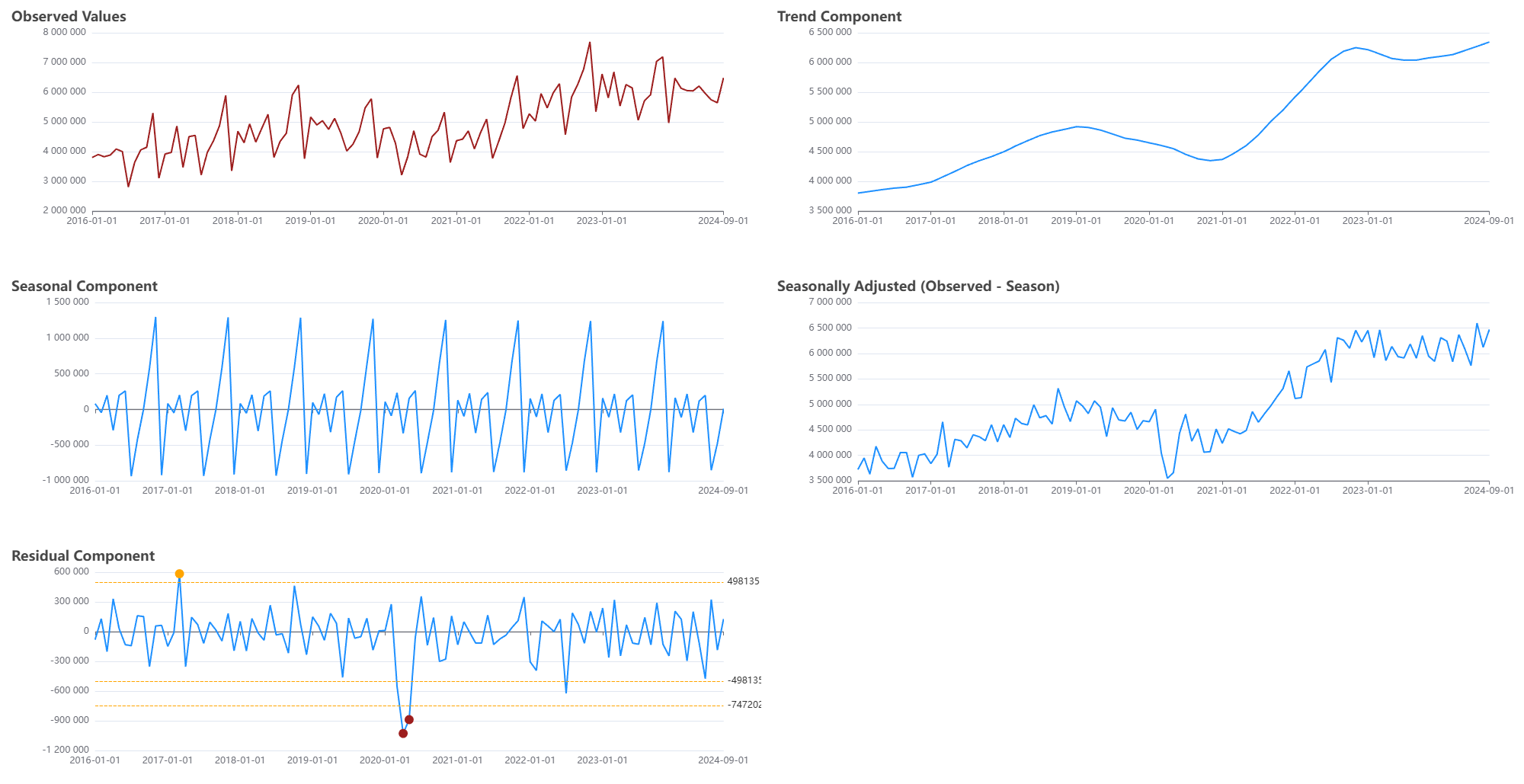
Automatically decomposes your data into trend, seasonal, and remainder components with interactive charts showing each element. Toggle between original, seasonally adjusted, and detrended views instantly.

Seasonal Variance Analysis

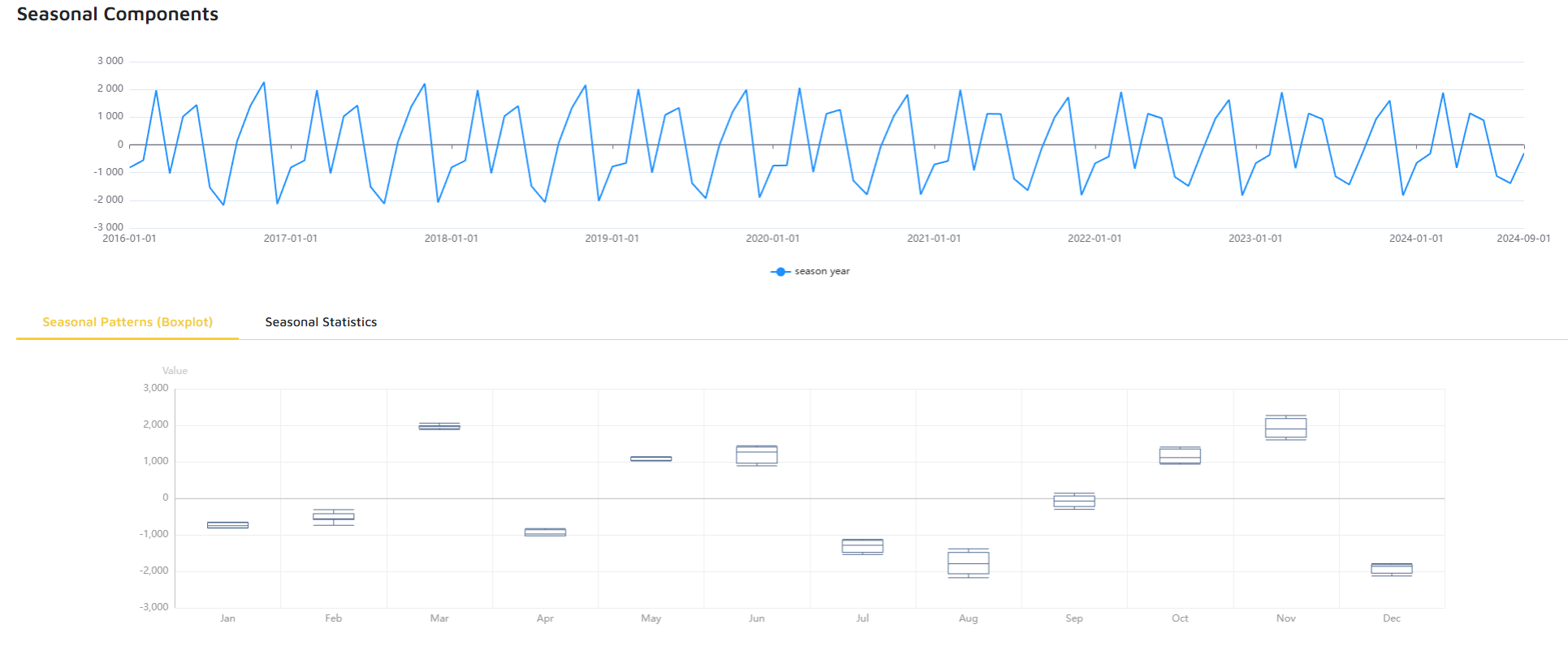
Visualizes variance across different time periods (monthly, weekly, daily) to identify high-risk seasonal windows requiring larger safety buffers or flexible capacity planning.

AI-Powered Explanations

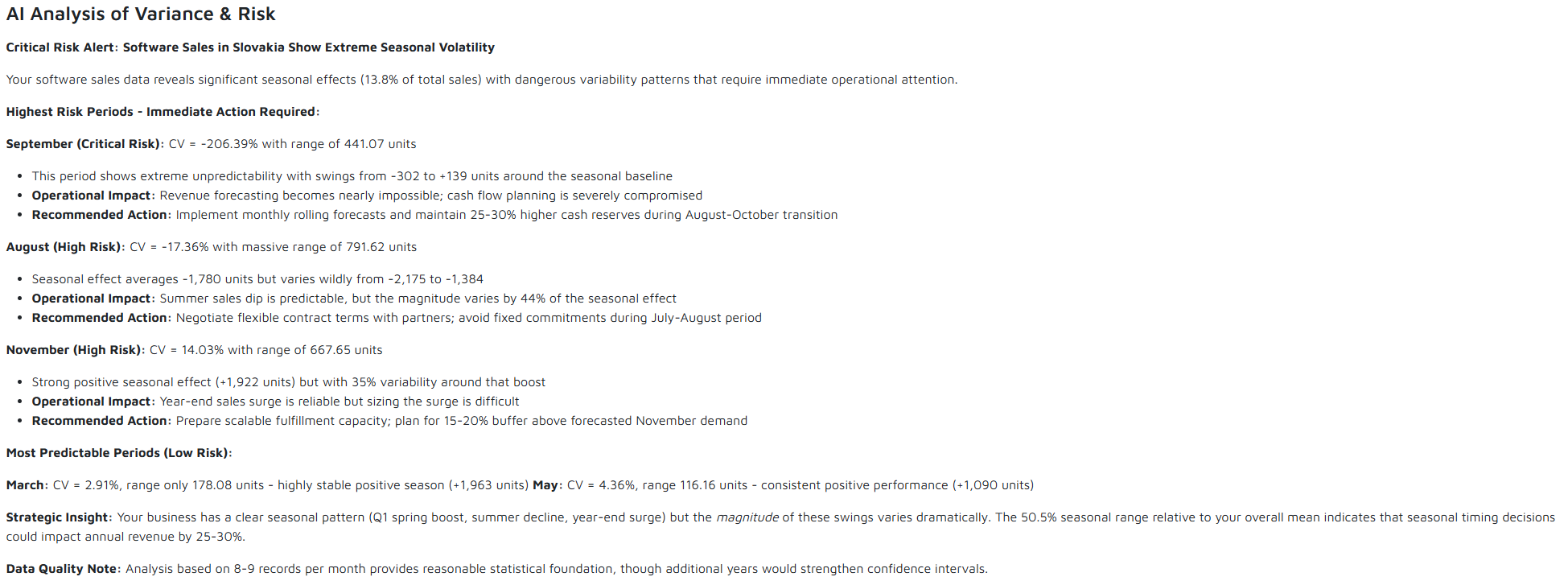
No statistics degree required. QuantixAI’s AI explains what the decomposition reveals about your business in plain language, highlighting key insights and actionable recommendations.

How QuantixAI Protects Your Data

Unlike generic AI tools that send your entire dataset to external servers, QuantixAI employs a privacy-first architecture. The system computes decomposition and statistical summaries locally, then sends only aggregated metrics (means, variances, seasonal indices) to the AI explanation engine. This means your raw sales data, customer information, and business details never leave your infrastructure – you get AI-powered insights without AI-powered privacy risks.

The chat-based interface allows natural follow-up questions: “Why is December variance so high?” “What’s causing that spike in the remainder component last quarter?” “How does this year’s trend compare to industry benchmarks?” Your tier determines available follow-ups (1 for basic, 3 for professional, unlimited for enterprise), but the underlying analysis remains consistent: comprehensive, accurate, and private.

Conclusion: From Data to Understanding

Time series analysis transforms business data from a historical record into strategic intelligence. The methods we’ve explored – MSTL decomposition, seasonal variance analysis, and rigorous year-over-year comparison – aren’t advanced statistics reserved for enterprise analytics teams. They’re practical tools that answer the fundamental questions every SME manager faces:

• Is my business actually growing, or am I just seeing seasonal fluctuations?
• Which time periods carry the most risk, requiring larger buffers and flexible capacity?
• How do I accurately compare performance across periods without seasonal distortion?
• What anomalies or patterns in my data require investigation or action?

The business value extends across every function. Inventory managers optimize stock levels based on both expected demand and variance. Financial controllers forecast cash flow using seasonally adjusted trends rather than hoping this December mirrors last December. Operations leaders schedule staff according to both peak volume and peak variability. Marketing teams time campaigns to seasonal windows showing both high demand and predictable patterns.

Understanding your data’s underlying dynamics – the trend showing where you’re headed, the seasonal patterns creating both opportunity and risk, and the remainder revealing anomalies – enables the kind of confident, evidence-based decisions that separate successful SMEs from those perpetually reacting to yesterday’s numbers. The question isn’t whether to invest in proper time series analysis, but how quickly you can start seeing your business through this clearer lens.

References

- Hyndman, R. J., & Athanasopoulos, G. (2021). Forecasting: Principles and Practice (3rd ed.). OTexts. Chapter 3: Time series decomposition. https://otexts.com/fpp3/decomposition.html
- Bandara, K., Hyndman, R. J., & Bergmeir, C. (2021). MSTL: A Seasonal-Trend Decomposition Algorithm for Time Series with Multiple Seasonal Patterns. arXiv preprint arXiv:2107.13462. https://arxiv.org/abs/2107.13462
- Emergent Mind. (2024). Biseasonal MSTL Model: Applications and Use Cases. https://www.emergentmind.com/topics/biseasonal-mstl-model
- Smart Software. (2024). 12 Causes of Overstocking and Practical Solutions. https://smartcorp.com/blog/12-causes-of-overstocking-and-practical-solutions/
- P. Pandey et al. (2021). Determining optimal workforce size and schedule at the retail store considering overstaffing and understaffing costs. Computers & Industrial Engineering https://doi.org/10.1016/j.omega.2021.102348
- Ren, Shuyun & Chan, Hau Ling & Siqin, Tana. (2020). Demand forecasting in retail operations for fashionable products: methods, practices, and real case study. Annals of Operations Research. 291. 10.1007/s10479-019-03148-8. https://www.researchgate.net/publication/330690606
- Toast POS. (2024). Restaurant Seasonality: How to Hire for Busy Season. https://pos.toasttab.com/blog/on-the-line/restaurant-seasonality-hiring
- Corporate Finance Institute. (2024). Year-Over-Year (YoY) Analysis. https://corporatefinanceinstitute.com/resources/accounting/year-over-year-yoy-analysis/
- National Retail Federation. (2026). 4-5-4 Calendar. https://nrf.com/resources/4-5-4-calendar
- FE Training. (2024). Year-Over-Year (YOY) Analysis and Best Practices. https://www.fe.training/free-resources/accounting/year-over-year-yoy/